Many use antenna-modelling packages to explore performance and undertake ‘what if’ studies. I have used EZNEC for many years, but there are other options.
For simple antenna structures (dipoles, verticals, end-fed wires etc) inputting wire-coordinates, segment counts, and so forth is relatively straightforward; there’s not much typing, changing wire lengths is easy.
That said, once we wish to model more-complex structures, the ‘data input’ workload starts to increase. For example, consider a 2-element Quad for the 2m band, with a driven-element (DE) and a reflector (REF).
Using pencil and paper, we make some initial estimates of DE and REF sizes. We have 8 wires that need to be appropriately connected to 8 spatial coordinates (x,y,z). The 4 REF wires are slightly longer than the 4 DE wires. And, is the (0,0,0) point to be at the centre of the DE bottom wire, the centre of the DE square, or perhaps the notional centre of the whole structure?
After several minutes typing, correction of a few mistakes, and a various other inputs, we are ready to run. The initial output shows the antenna to be resonant around 147.7MHz, nowhere near our 145.0MHz design figure; and the front-to-back (F/B) looks poor relative to text-book figures.
As such, the DE and REF lengths need to increase to move down the band; the poor F/B may be a DE-REF spacing issue, and/or an issue with the DE and REF relative sizes.
All the wire lengths need to change, together with all the spatial coordinates, in fact almost every figure in the input grid will be different. Having used pencil and paper to re-calculate lengths and coordinates, several minutes of tedious typing are required to input the new data.
A second run shows the resonant frequency to be 145.9MHz; still too high. And the F/B doesn’t seem that much better.
How many rounds of ‘rinse and repeat’ are you up for?
Not too many I imagine. But, thankfully, there is a better way.
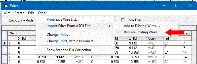
Buried deep inside the EZNEC manual is an explanation of how to automate the inputting of ‘Wires’ data. The image below shows the menu entry in the ‘Wires’ dialog box. Choose: Other | Import Wires From ASCII File | Replace Existing Wires…
We need to make the ASCII file (which must have CR/LF line-endings, not just LF). The format is:
; comment-line(s)
;
FT IN ← the required units
x1,y1,z1,x2,y2,z2,thickness,#segments ← wire coords, thickness, seg count
Each wire requires its own row. Below you will find a full example.
Using your favourite programming language - Python, Java, C, Rust, Fortran, 64-bit ARM assembly, or whatever, you can readily automate the production of these ASCII ‘Wires’ files.
Starting with a chosen frequency, computing all the wire lengths, arrangements and coordinates is no more than High-school geometry.
So now, even if we require 23 iterations of ‘rinse and repeat’ to reach our preferred solution, the whole workflow is relatively painless.
Apologies to the many (few?) who knew this already.
73 Dave
PS For those without O-level Latin, ‘Non vi, sed arte’ = ‘Not by force, by guile’, the motto of the Long-Range Desert Group.
; 2m 2-el quad v1.00
FT IN
0.000,0.000,24.142,0.000,0.858,24.142,0.1,7
0.000,0.000,24.142,0.000,-0.858,24.142,0.1,7
0.000,0.858,24.142,0.000,0.858,25.858,0.1,14
0.000,-0.858,24.142,0.000,-0.858,25.858,0.1,14
0.000,0.858,25.858,0.000,-0.858,25.858,0.1,14
-0.780,0.901,24.099,-0.780,-0.901,24.099,0.1,14
-0.780,0.901,24.099,-0.780,0.901,25.901,0.1,14
-0.780,-0.901,24.099,-0.780,-0.901,25.901,0.1,14
-0.780,0.901,25.901,-0.780,-0.901,25.901,0.1,14


 1984")